
StoJ, an implementation of Stochastic Join
Wed 15 Sep 2004 00:02 BST

Well, since I wrote about some of the issues in stochastic-π based biological modelling, I’ve had a little spare time, a little inspiration, and a supportive workplace environment (thanks again, LShift!), and I’ve implemented StoJ, a polyadic, asynchronous stochastic π calculus with input join and no summation. Rates are associated with a join, not with a channel. I implemented Gillespie’s “first reaction” method (it seemed simplest — and despite its inefficiency it’s performing reasonably well, although I suspect I have Moore’s “law” to thank for that more than anything else).
I used OCaml as the implementation language — the parsing tools are quite smooth and good to work with — and gnuplot to graph the output of each simulation run. This is my first OCaml project, and I’m finding it quite pleasant despite the syntax.
Here’s an example model in StoJ. I duplicated the rates and the overall design of the model from the Clock.zip code archive at the BioSPI website. This model is discussed in Aviv Regev’s paper “Representation and simulation of molecular pathways in the stochastic π-calculus.” The implementation of the model below gives the same output graphs as Regev’s model gives, which is a nice confirmation of the model and of the StoJ system itself.
// Circadian clock model
// Based on Regev et al

new
        DNA_a, DNA_r,
        !MRNA_a, !MRNA_r,
        !protein_a, !protein_r,
        DNA_a_promoted, DNA_r_promoted,
        !complex_ar . (

// Start state.
DNA_a<> | DNA_r<>

// Basal rate transcription.
| rec L. DNA_a() ->[4]       (DNA_a<> | MRNA_a<> | L)
| rec L. DNA_r() ->[0.001]   (DNA_r<> | MRNA_r<> | L)

// MRNA degradation.
| rec L. MRNA_a() ->[1.0]    (L)
| rec L. MRNA_r() ->[0.02]   (L)

// Translation.
| rec L. MRNA_a() ->[1.0]    (MRNA_a<> | protein_a<> | L)
| rec L. MRNA_r() ->[0.1]    (MRNA_r<> | protein_r<> | L)

// Protein degradation.
| rec L. protein_a() ->[0.1] (L)
| rec L. protein_r() ->[0.01]        (L)

// A/R Complex formation.
| rec L. protein_a() & protein_r() ->[100.0]     (complex_ar<> | L)

// A/R Complex degradation.
| rec L. complex_ar() ->[0.1]        (protein_r<> | L)
| rec L. complex_ar() ->[0.01]       (protein_a<> | L)

// Activator binding/unbinding to A promoter, and enhanced transcription
| rec L. protein_a() & DNA_a() ->[10]    (DNA_a_promoted<> | L)
| rec L. DNA_a_promoted() ->[10]         (protein_a<> | DNA_a<> | L)
| rec L. DNA_a_promoted() ->[40]         (DNA_a_promoted<> | MRNA_a<> | L)

// Activator binding/unbinding to R promoter, and enhanced transcription
| rec L. protein_a() & DNA_r() ->[10]    (DNA_r_promoted<> | L)
| rec L. DNA_r_promoted() ->[100]        (protein_a<> | DNA_r<> | L)
| rec L. DNA_r_promoted() ->[2]          (DNA_r_promoted<> | MRNA_r<> | L)

)
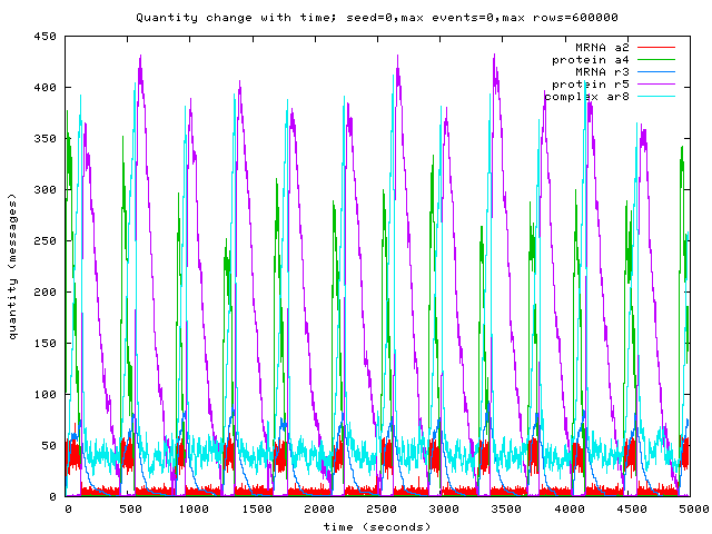
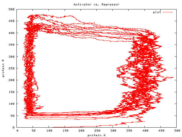
Here are a couple of graphs produced by the simulator from the program above — first a graph of reagent concentrations varying with time, and then a graph of Repressor (R) molecule concentration against Activator (A) molecule concentration, showing the bistable nature of the whole system. If you take a look at the graphs in Regev’s paper, you’ll see that the spikes in reagent concentration occur in the same places with the same frequency in our model as in Regev’s.
I also implemented a simple Java applet/application that uses a (human-assisted) mass-spring layout to draw a graph of the (statically apparent) dataflow in the StoJ program it takes as input. It still needs a bit of refining — the graphs/programs tend to be quite densely connected in places, and not only is mass-spring layout poor at densely-connected graphs, especially with cycles, but it doesn’t identify any potential clustering in the graph either. I get the feeling clustering (subgraphs) will be important for visualising dataflow in larger models.
Here’s a simple chemical equilibrium model in StoJ:
// A simple H + Cl <--> HCl model,
// similar to that in Andrew Phillips' slides
// with numbers taken from his slides.
// See http://www.doc.ic.ac.uk/~anp/spim/Slides.pdf
// page 16.

new !h, !cl, !hcl . (
  rec ASSOC.  h() & cl() ->[100] (hcl<> | ASSOC)
| rec DISSOC. hcl() ->[10] (h<> | cl<> | DISSOC)
| h<> * 100 | cl<> * 100
)
And here’s the display generated by the Java program visualisation application:
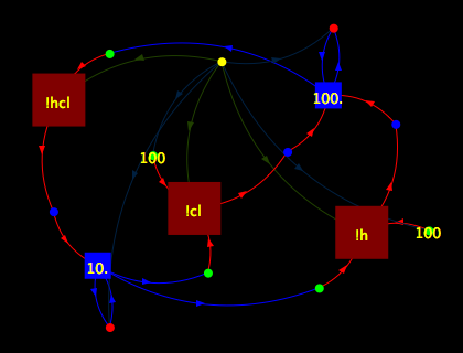
As you can imagine, for larger models the display gets cluttered quite quickly. A note on implementation though - I found Java2D to be surprisingly pleasant to work with. The built-in support for double-buffering of JComponents along with the various classes of Shape helped me quickly develop the application.